지도에서 시각적으로 표시 할 수있는 물리적 객체 외에도 SWMM은 여러 비 시각적 데이터 객체 클래스를 사용하여 연구 영역 내에서 추가 특성 및 프로세스를 설명한다.

기후학

온도

대기 온도 데이터는 유출수 계산 중 강설 및 설상 프로세스를 시뮬레이션 할 때 사용된다. 또한 일일 증발 률을 계산하는 데 사용할 수 있다. 이러한 프로세스가 시뮬레이트되지 않으면 온도 데이터가 필요하지 않습니다. 다음 소스 중 하나에서 대기 온도 데이터를 SWMM에 공급할 수 있다.

• 포인트 값의 사용자 정의 시계열 (중간 시간의 값이 보간된다)
• 일별 최소값과 최대 값을 포함하는 외부 기후 파일 (SWMM은 해당 연도의 날짜에 따라 이러한 값을 통해 사인 커브 곡선에 맞 춥니 다).

사용자가 정의한 시계열의 경우 온도는 미국 단위는 F이고 미터법 단위는 C이다. 외부 기후 파일은 증발 및 풍속을 직접 공급하는 데에도 사용할 수 있다.

 

증발

지하층 대수층의 지하수, 열린 통로를 흐르는 물 및 저류지에 보관 된 물에 대해 증발이 일어날 수있다. 증발 률은 다음과 같이 나타낼 수 있다.

• 하나의 상수 값
• 월평균 값 집합
• 사용자가 정의한 값의 시계열
• 외부 기후 파일에 포함 된 일별 기온으로부터 계산 된 값
• 외부 기후 파일에서 직접 읽은 일일 값

기후 파일에서 직접 비율을 판독할 경우 팬 증발 데이터를 자유 수표면으로 변환하기 위해 일련의 월별 팬 계수를 제공해야한다. 또한 옵션이 있어 강수량이 없는 기간 동안에만 증발이 가능하다.

SWMM에 공급되는 증발 률은 잠재적 인 비율이라는 점에 유의해야 한다.  증발 된 실제 물의 양은 이용 가능한 물의 양에 달려 있다.

 

풍속

풍속은 융설 계산에만 사용되는 선택적인 기후 변수이다. SWMM은 일일 최소 / 최대 온도에 사용되는 동일한 기후 파일에 포함 된 월간 평균 속도 또는 풍속 데이터를 사용할 수 있다.

 

융설

융설 매개 변수는 강설량과 융설를 시뮬레이션 할 때 전체 연구 영역에 적용되는 기후 변수이다. 그들은 다음을 포함한다.

• 강수량이 눈으로 내리는 기온
• 눈 표면의 열교환 특성
• 학습 영역 고도, 위도 및 경도 보정

 

면적감소

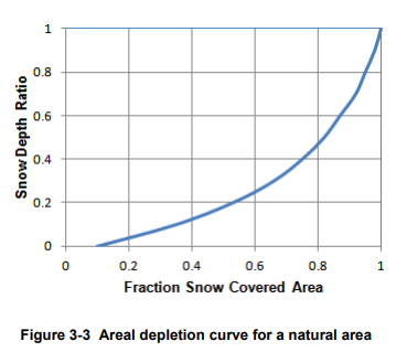
면적 감소는 축적 된 눈이 소유역의 표면에서 불균일하게 녹는 경향을 말한다. 녹는 과정이 진행됨에 따라 눈으로 덮인 면적이 줄어 든다. 이 현상은 눈이 남아있는 총 면적의 비율을 눈 깊이 100 %가있는 실제 눈 깊이의 비율에 대해 적용한 면적 감소 곡선에 의해 설명된다. 자연 영역에 대한 일반적인 ADC가 그림 3-3에 나와 있다. SWMM에는 두 개의 곡선이 제공 될 수 있다. 하나는 불 침투성 영역이고 다른 하나는 투과성 영역이다.

 

기후 조정

기후 조정은 SWMM이 시뮬레이션의 각 단계에서 달리 사용하는 온도, 증발 률 및 강우 강도에 적용되는 선택적 수정이다. 월별로 주기적으로 변화하는 별도의 조정 세트를 이러한 변수에 할당 할 수 있다. 원래의 기후 시계열을 수정하지 않고도 미래 기후 변화의 영향을 조사 할 수있는 간단한 방법을 제공한다.

비슷한 방식으로, 일련의 월별 조정은 기존 대지 표면에서의 강우 침투와 저장 노드와 관거에서의 유출을 계산하는 데 사용되는 유압 전도도에 적용될 수 있다. 이는 온도 상승과 함께 유압 전도성의 증가를 반영할 수 있으며, 동결 지반과 같은 지반 표면 조건의 계절적 변화가 침투 용량에 영향을 미칠 수 있다.

 

 

스노우 팩

스노우 팩 객체에는 소유역 내의 세 가지 유형의 하위 영역에 대한 눈의 형성, 제거 및 녹을 특성화하는 매개 변수가 있다.

• Plowable 스노우 팩 영역은 전체 불 투과성 영역의 사용자 정의 부분으로 구성된다. 그것은 제설기로 제설 작업을 할 수있는 거리와 주차장과 같은 구역을 나타 내기위한 것이다.
• 불 투수 제설 포장 구역은 소유역의 남아있는 불 투수 지역을 덮고 있다.
• 투명한 적설 구역은 소유역의 전체 투수 지역을 포함한다.

이 세 영역 각각은 다음 매개 변수로 특징 지어진다.

• 최소 및 최대 융설 계수
• 융설을 위한 최소 기온
• snow depth above which 100% areal coverage occurs
• 초기 눈 깊이
• 팩의 초기 및 최대 물 함량

In addition, a set of snow removal parameters can be assigned to the Plowable area. These parameters consist of the depth at which snow removal begins and the fractions of snow moved onto various other areas.

Subcatchments are assigned a snow pack object through their Snow Pack property. A single snow pack object can be applied to any number of subcatchments. Assigning a snow pack to a subcatchment simply establishes the melt parameters and initial snow conditions for that subcatchment. Internally, SWMM creates a “physical” snow pack for each subcatchment, which tracks snow accumulation and melting for that particular subcatchment based on its snow pack parameters, its amount of pervious and impervious area, and the precipitation history it sees.

 

 

대수층

Aquifers are sub-surface groundwater zones used to model the vertical movement of water infiltrating from the subcatchments that lie above them. They also permit the infiltration of groundwater into the drainage system, or exfiltration of surface water from the drainage system, depending on the hydraulic gradient that exists. Aquifers are only required in models that need to explicitly account for the exchange of groundwater with the drainage system or to establish base flow and recession curves in natural channels and non-urban systems. The parameters of an aquifer object can be shared by several subcatchments but there is no exchange of groundwater between subcatchments. A drainage system node can exchange groundwater with more than one subcatchment.

Aquifers are represented using two zones – an un-saturated zone and a saturated zone. Their behavior is characterized using such parameters as soil porosity, hydraulic conductivity, evapotranspiration depth, bottom elevation, and loss rate to deep groundwater. In addition, the initial water table elevation and initial moisture content of the unsaturated zone must be supplied.

Aquifers are connected to subcatchments and to drainage system nodes through a subcatchment’s Groundwater Flow property. This property also contains parameters that govern the rate of groundwater flow between the aquifer’s saturated zone and the drainage system node.

 

 

단위유량도

Unit Hydrographs (UHs) estimate rainfall-dependent infiltration/inflow (RDII) into a sewer system. A UH set contains up to three such hydrographs, one for a short-term response, one for an intermediate-term response, and one for a long-term response. A UH group can have up to 12 UH sets, one for each month of the year. Each UH group is considered as a separate object by SWMM, and is assigned its own unique name along with the name of the rain gage that supplies rainfall data to it.

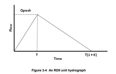
Each unit hydrograph, as shown in Figure 3-4, is defined by three parameters:

• R: the fraction of rainfall volume that enters the sewer system
• T: the time from the onset of rainfall to the peak of the UH in hours
• K: the ratio of time to recession of the UH to the time to peak

Each unit hydrograph can also have a set of Initial Abstraction (IA) parameters associated with it. These determine how much rainfall is lost to interception and depression storage before any excess rainfall is generated and transformed into RDII flow by the hydrograph. The IA parameters consist of:

• a maximum possible depth of IA (inches or mm),
• a recovery rate (inches/day or mm/day) at which stored IA is depleted during dry periods,
• an initial depth of stored IA (inches or mm)

To generate RDII into a drainage system node, the node must identify (through its Inflows property) the UH group and the area of the surrounding sewershed that contributes RDII flow.

An alternative to using unit hydrographs to define RDII flow is to create an external RDII interface file, which contains RDII time series data. See Section 11.7 Interface Files.

Unit hydrographs could also be used to replace SWMM’s main rainfall-runoff process that uses Subcatchment objects, provided that properly calibrated UHs are utilized. In this case what SWMM calls RDII inflow to a node would actually represent overland runoff.

횡단면

Transects refer to the geometric data that describe how bottom elevation varies with horizontal distance over the cross section of a natural channel or irregular-shaped conduit. Figure 3-5 displays an example transect for a natural channel.

Each transect must be given a unique name. Conduits refer to that name to represent their shape. A special Transect Editor is available for editing the station-elevation data of a transect. SWMM internally converts these data into tables of area, top width, and hydraulic radius versus channel depth. In addition, as shown in Figure 3-5, each transect can have a left and right overbank section whose Manning’s roughness can be different from that of the main channel. This feature can provide more realistic estimates of channel conveyance under high flow conditions.

 

 

외부 유입유량

In addition to inflows originating from subcatchment runoff and groundwater, drainage system nodes can receive three other types of external inflows:

• Direct Inflows – These are user-defined time series of inflows added directly into a node. They can be used to perform flow and water quality routing in the absence of any runoff computations (as in a study area where no subcatchments are defined).
• Dry Weather Inflows – These are continuous inflows that typically reflect the contribution from sanitary sewage in sewer systems or base flows in pipes and stream channels. They are represented by an average inflow rate that can be periodically adjusted on a monthly, daily, and hourly basis by applying Time Pattern multipliers to this average value.
• Rainfall-Dependent Infiltration/Inflow (RDII) – These are stormwater flows that enter sanitary or combined sewers due to “inflow” from direct connections of downspouts, sump pumps, foundation drains, etc. as well as “infiltration” of subsurface water through cracked pipes, leaky joints, poor manhole connections, etc. RDII can be computed for a given rainfall record based on set of triangular unit hydrographs (UH) that determine a short-term, intermediate-term, and long-term inflow response for each time period of rainfall. Any number of UH sets can be supplied for different sewershed areas and different months of the year. RDII flows can also be specified in an external RDII interface file.

Direct, Dry Weather, and RDII inflows are properties associated with each type of drainage system node (junctions, outfalls, flow dividers, and storage units) and can be specified when nodes are edited. They can be used to perform flow and water quality routing in the absence of any runoff computations (as in a study area where no subcatchments are defined). It is also possible to make the outflows generated from an upstream drainage system be the inflows to a downstream system by using interface files. See Section 11.7 for further details.

 

 

제어 규칙

Control Rules determine how pumps and regulators in the drainage system will be adjusted over the course of a simulation. Some examples of these rules are:

Simple time-based pump control:
RULE R1
IF SIMULATION TIME > 8
THEN PUMP 12 STATUS = ON
ELSE PUMP 12 STATUS = OFF

 

Multiple-condition orifice gate control:
RULE R2A
IF NODE 23 DEPTH > 12
AND LINK 165 FLOW > 100
THEN ORIFICE R55 SETTING = 0.5

RULE R2B
IF NODE 23 DEPTH > 12
AND LINK 165 FLOW > 200
THEN ORIFICE R55 SETTING = 1.0

RULE R2C
IF NODE 23 DEPTH <= 12
OR LINK 165 FLOW <= 100
THEN ORIFICE R55 SETTING = 0

 

Pump station operation:
RULE R3A
IF NODE N1 DEPTH > 5
THEN PUMP N1A STATUS = ON

RULE R3B
IF NODE N1 DEPTH > 7
THEN PUMP N1B STATUS = ON

RULE R3C
IF NODE N1 DEPTH <= 3
THEN PUMP N1A STATUS = OFF
AND PUMP N1B STATUS = OFF
Modulated weir height control:
RULE R4
IF NODE N2 DEPTH >= 0
THEN WEIR W25 SETTING = CURVE C25

 

 

오염 물질

SWMM can simulate the generation, inflow and transport of any number of user-defined pollutants. Required information for each pollutant includes:

• pollutant name
• concentration units (i.e., milligrams/liter, micrograms/liter, or counts/liter)
• concentration in rainfall
• concentration in groundwater
• concentration in inflow/infiltration
• concentration in dry weather flow
• initial concentration throughout the conveyance system
• first-order decay coefficient.

Co-pollutants can also be defined in SWMM. For example, pollutant X can have a co-pollutant Y, meaning that the runoff concentration of X will have some fixed fraction of the runoff concentration of Y added to it.

Pollutant buildup and washoff from subcatchment areas are determined by the land uses assigned to those areas. Input loadings of pollutants to the drainage system can also originate from external time series inflows as well as from dry weather inflows.

 

 

토지 이용

토지 이용은 소유역에 할당 된 개발 활동 또는 지표면 특성의 범주이다. 토지 이용 활동의 예는 주거용, 상업용, 산업 및 개발되지 않은 활동이다. 지표면 특성에는 옥상, 잔디, 포장 도로, 평온한 토양 등이 포함될 수 있다. 토지 이용은 오염원 축적의 공간적 변화와 소유역 내의 씻기 율을 설명하기 위해서만 사용된다.

SWMM 사용자는 토지 용도를 정의하고 소유역 영역에 할당하는 많은 옵션을 제공한다. 하나의 접근법은 각 소유역에 대한 토지 용도의 혼합을 할당하는 것인데, 이는 소유 역내의 모든 토지 이용이 동일한 이전 및 불투수 한 특성을 갖는 결과를 가져온다. 또 다른 접근법은 분류를 반영하는 투수 속성과 불투수 한 특성의 집합과 함께 단일 토지 이용 분류를 갖는 소유역을 만드는 것이다.

각 토지 이용 범주에 대해 다음 절차를 정의할 수 있다.

• 오염물 축적
• 오염물 세척
• 거리 청소

 

오염 물질 축적

Pollutant buildup that accumulates within a land use category is described (or “normalized”) by either a mass per unit of subcatchment area or per unit of curb length. Mass is expressed in pounds for US units and kilograms for metric units. The amount of buildup is a function of the number of preceding dry weather days and can be computed using one of the following functions:

Power Function: Pollutant buildup (B) accumulates proportionally to time (t) raised to some power, until a maximum limit is achieved,

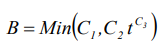
where C1 = maximum buildup possible (mass per unit of area or curb length), C2 = buildup rate constant, and C3 = time exponent.

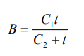
Exponential Function: Buildup follows an exponential growth curve that approaches a maximum limit asymptotically,

where C1 = maximum buildup possible (mass per unit of area or curb length) and C2 = buildup rate constant (1/days).

Saturation Function: Buildup begins at a linear rate that continuously declines with time until a saturation value is reached,

where C1 = maximum buildup possible (mass per unit area or curb length) and C2 = half-saturation constant (days to reach half of the maximum buildup).

External Time Series: This option allows one to use a Time Series to describe the rate of buildup per day as a function of time. The values placed in the time series would have units of mass per unit area (or curb length) per day. One can also provide a maximum possible buildup (mass per unit area or curb length) with this option and a scaling factor that multiplies the time series values.

 

오염 물질 세척

Pollutant washoff from a given land use category occurs during wet weather periods and can be described in one of the following ways:

Exponential Washoff: The washoff load (W) in units of mass per hour is proportional to the product of runoff raised to some power and to the amount of buildup remaining,

where C1 = washoff coefficient, C2 = washoff exponent, q = runoff rate per unit area (inches/hour or mm/hour), and B = pollutant buildup in mass units. The buildup here is the total mass (not per area or curb length) and both buildup and washoff mass units are the same as used to express the pollutant’s concentration (milligrams, micrograms, or counts).

Rating Curve Washoff: The rate of washoff W in mass per second is proportional to the runoff rate raised to some power,

where C1 = washoff coefficient, C2 = washoff exponent, and Q = runoff rate in user-defined flow units.

Event Mean Concentration: This is a special case of Rating Curve Washoff where the exponent is 1.0 and the coefficient C1 represents the washoff pollutant concentration in mass per liter (Note: the conversion between user-defined flow units used for runoff and liters is handled internally by SWMM).

Note that in each case buildup is continuously depleted as washoff proceeds, and washoff ceases when there is no more buildup available.

Washoff loads for a given pollutant and land use category can be reduced by a fixed percentage by specifying a BMP Removal Efficiency that reflects the effectiveness of any BMP controls associated with the land use. It is also possible to use the Event Mean Concentration option by itself, without having to model any pollutant buildup at all.

 

거리 청소

Street sweeping can be used on each land use category to periodically reduce the accumulated buildup of specific pollutants. The parameters that describe street sweeping include:

• days between sweeping
• days since the last sweeping at the start of the simulation
• the fraction of buildup of all pollutants that is available for removal by sweeping
• the fraction of available buildup for each pollutant removed by sweeping

Note that these parameters can be different for each land use, and the last parameter can vary also with pollutant.

 

 

수처리

임의의 배수 시스템 노드로 유입되는 흐름 스트림으로부터의 오염물 제거는 일련의 처리 기능을 노드에 할당함으로써 모델링된다. 처리 함수는 다음과 관련된 잘 구성된 수학적 표현 일 수 있다.

• 오염 물질 농도
• 다른 오염 물질의 제거
• 유량, 깊이, 수리 학적 체류 시간 등과 같은 여러 프로세스 변수 중 하나, 기타

처리 기능의 결과는 농도 (문자 C로 표시) 또는 부분 제거 (R로 표시) 중 하나 일 수 있니다. 예를 들어, 저류 노드에서 나가는 BOD의 1 차 감쇠 표현식은 다음과 같이 표현 될 수 있다.

C = BOD * exp(-0.05 * HRT)

여기서 HRT는 수리 학적 체류 시간에 대해 예약 된 변수 이름이다. 총 부유 물질 (TSS)의 제거에 비례하는 일부 미량 오염 물질의 제거는 다음과 같이 표현 될 수있다.

R = 0.75 * R_TSS

 

 

커브

커브 객체는 두 수량 간의 기능적 관계를 설명하는 데 사용됩니다. SWMM에서 사용되는 곡선 유형은 다음과 같다.

• Storage – 저류 장치 노드의 표면적이 수심에 따라 어떻게 달라지는 지 설명한다.
• Shape – 사용자 정의 단면 형상의 너비가 관거 링크 높이에 따라 어떻게 달라지는 지 설명한다.
• Diversion – 유량 분배 노드에서 유출 된 유출을 총 유입량과 관련 시킨다.
• Tidal – 배출구 노드의 수위가 하루 중 시간별로 어떻게 변하는 지 설명한다.
• Pump – 펌프 링크를 통과하는 흐름을 업스트림 노드의 깊이 또는 체적 또는 펌프가 전달한 수두에 관련 시킨다.
• Rating – relates flow through an Outlet link to the freeboard depth or head difference across the outlet.
• Control – determines how the control setting of a pump or flow regulator varies as a function of some control variable (such as water level at a particular node) as specified in a Modulated Control rule.

Each curve must be given a unique name and can be assigned any number of data pairs.

 

 

시계열

시계열 개체는 특정 개체 속성이 시간에 따라 어떻게 변하는 지 설명하는 데 사용된다. 시계열을 사용하여 다음을 설명 할 수 있다.

• 온도 자료
• 증발 자료
• 강수량 자료
• 배출구 노드의 수위
• 배수 시스템 노드에서 외부 유입 수문곡선
• 배수 시스템 노드에서 외부 유입 오염곡선
• 펌프 및 유량 조절기에 대한 제어 설정

각 시계열은 고유 한 이름을 부여 받아야하며 여러 개의 시간 – 값 데이터 쌍을 지정할 수 있다. 시간은 시뮬레이션을 시작한 후 몇 시간 또는 절대 날짜와 시간으로 지정할 수 있다. 시계열 데이터는 프로그램에 직접 입력하거나 사용자가 제공 한 시계열 파일에서 액세스 할 수 있다.

강우 시간 시리즈의 경우, 강우량이 0이 아닌 기간을 입력하기 만하면된다. SWMM은 강우량 값을 시계열을 사용하는 강우 계기에 지정된 기록 간격 동안 지속되는 상수 값으로 해석한다. 다른 모든 유형의 시계열의 경우 SWMM은 보간을 사용하여 기록 된 값 사이의 시간에 값을 추정한다.

시계열의 범위를 벗어나는 시간의 경우, SWMM은 강우량 및 외부 유입 시간 시리즈에 대해 0 값을 사용하고 온도, 증발 및 수위 시계열에 대한 첫 번째 또는 마지막 시리즈 값을 사용한다.

 

 

시간 패턴

시간 패턴을 사용하면 외부 건기 유량 (DWF)을 주기적으로 변경할 수 있다. 기본 DWF 유속 또는 오염 물질 농도에 대한 승수로 적용되는 일련의 조정 요인으로 구성됩니다. 시간 패턴의 다른 유형은 다음과 같다.

Monthly – 연중 매월 하나의 승수
Daily – 일주일마다 하나의 승수
Hourly – 오전 12 시부 터 오후 11 시까 지 매 시간마다 하나의 승수
Weekend – 주말에 대한 시간별 승수

각 시간 패턴에는 고유 한 이름이 있어야하며 만들 수있는 패턴의 수에는 제한이 없다. 각각의 건기 유입 (유량 또는 수질)은 위에 나열된 각 유형별로 최대 4 가지 패턴을 가질 수 있다.

 

 

LID 제어

LID 제어는 표면 유출수를  저류, 침투 및 증발산의 일부 조합을 제공하도록 고안된 저 영향개발 기법이다. 그들은 대수층 및 스노우팩을 처리하는 것과 마찬가지로 주어진 소유역의 속성으로 간주된다. SWMM은 LID 컨트롤의 8 가지 일반 유형을 명시 적으로 모델링 할 수 있다.

식생 체류 장치(Bio-retention Cells)는 자갈 배수 장치 위에 놓인 인공 토양 혼합물에서 자라는 식물을 포함하는 저류 시설이다.  주변 지역에서 포착 된 직접 강우와 유출의 저장, 침투 및 증발을 제공한다.

 

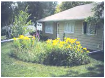빗물 정원(Rain Gardens)은 자갈층이 없이 토양층으로 구성된 식생 체류 장치 일종이다.

 

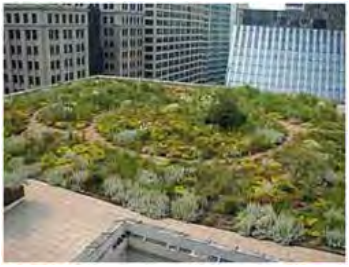옥상 녹화(Green Roofs)는 지붕에서 여과된 강우량을 대상으로 특수 배수 매트 재료 위에 놓이는 토양 층을 가진 식생 체류 장치의 또 다른 변형입니다.

 

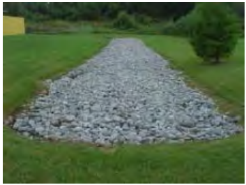침투 트렌치(Infiltration Trenches)는 자갈로 채워진 좁은 도랑형태로 경사지의 상류 불투수 지역의 유출량을 가로 채는 역할을 한다.  수집된 유량이 아래의 토양에 침투 할 수 있도록 저장량과 추가 시간을 제공한다.

 

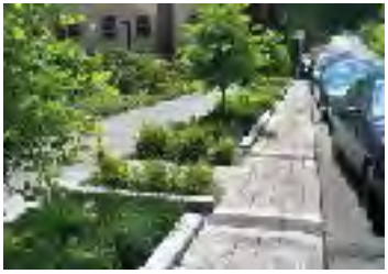
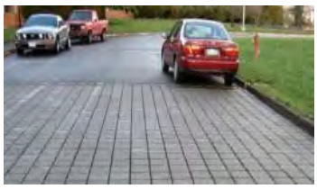연속 투수성 포장(Continuous Permeable Pavement systems )은 다공성 콘크리트 또는 아스팔트 혼합물로 포장 또는 자갈로 대상 지역을 채우고 유량이 바닥을 통해 침투할 수 있도록 설계된 시스템이다.

 

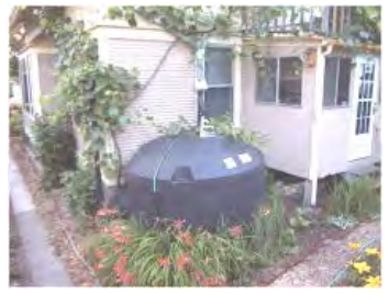빗물통(Rain Barrels)은 폭풍이 치는 동안 지붕 빗물을 모으고 건조한 기간에 빗물을 방출하거나 재사용 할 수있는 있다.

 

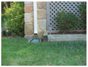옥상 연결 시설(Rooftop Disconnection)은 빗물 배수구로 직접 들어가는 대신 기존의 토지가 깔린 지역과 잔디밭으로 배출된다.  그것은 또한 투수 지역으로 넘쳐 흐르는 직접 연결된 배수구를 가진 지붕을 모델링 할 수 있다.

 

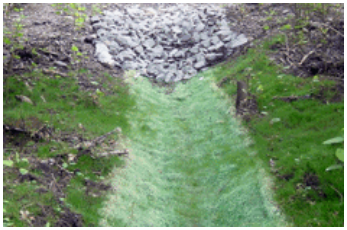식생 수로(Vegetative Swales )는 풀 또는 식생으로 덮인 경사지 형태로 우수의 운반을 늦추고 토양에 침투할 시간을 더 많이 준다.

 

식생 체류 장치, 침투 트렌치 및 투수성 포장은 과도한 저류된 유출을 현장에서 운반하고 장치가 침수하는 것을 방지하기 위해 자갈 저장 층에 선택적 배수 시스템을 포함 할 수 있습니다. 또한 토양 침투를 방지 할 수있는 불 침투성 바닥이나 층이 있을 수 있다. 침투 트렌치 및 투수성 포장은 막힘으로 인해 시간 경과에 따른 수리 전도도가 저하 될 수 있습니다.

일부 LID 실행은 상당한 오염 물질 배출 감소 혜택을 제공 할 수 있지만, 현재 SWMM은 유출 유량 감소로 인한 유출 질량 부하 감소를 모델링할 뿐이다.

소유역 내에 LID 통제를 배치하는 데는 두 가지 접근 방식이 있다.

• 소유역과 동일한 양의 비 LID 영역을 대체 할 기존 소유역에 하나 이상의 통제 장치를 배치한다.
• 새 소유역에 하나의 LID를 생성한다.

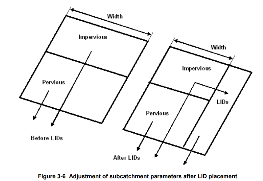
The first approach allows a mix of LIDs to be placed into a subcatchment, each treating a different portion of the runoff generated from the non-LID fraction of the subcatchment. Note that under this option the subcatchment’s LIDs act in parallel — it is not possible to make them act in series (i.e., have the outflow from one LID control become the inflow to another LID). Also, after LID placement the subcatchment’s Percent Impervious and Width properties may require adjustment to compensate for the amount of original subcatchment area that has now been replaced by LIDs (see Figure 3-6 below). For example, suppose that a subcatchment which is 40% impervious has 75% of that area converted to a permeable pavement LID. After the LID is added the subcatchment’s percent imperviousness should be changed to the percent of impervious area remaining divided by the percent of non-LID area remaining. This works out to (1 – 0.75)*40 / (100 – 0.75*40) or 14.3 %.

첫 번째 접근법은 LID의 혼합이 소유역에 놓일 수있게하며, 각각은 소유역의 비 LID 부분에서 생성 된 유출의 다른 부분을 처리한다. 이 옵션에서는 소유역의 LID가 병렬로 작동하므로 일련의 기능을 수행 할 수 없다 (즉, 하나의 LID 컨트롤에서 유입되는 유입 물이 다른 LID로 유입되도록). 또한 LID 배치 후 소유역의 퍼센트 불 투과성 및 폭 속성은 현재 LID로 대체 된 원래 소유역 면적을 보완하기 위해 조정이 필요할 수 있다 (아래 그림 3-6 참조). 예를 들어, 40 % 불 투수인 소유역이 그 지역의 75 %를 투과성 포장 도로 LID로 변환했다고 가정한다. 뚜껑을 추가 한 후에는 소유역의 불 침투성을 남은 비 침입 영역의 비율을 남은 비 LID 비율로 나눈 값으로 변경해야한다. 이것은 (1 – 0.75) * 40 / (100 – 0.75 * 40) 또는 14.3 %로 계산된다.

Under this first approach the runoff available for capture by the subcatchment’s LIDs is the runoff generated from its impervious area. If the option to re-route some fraction of this runoff to the pervious area is exercised, then only the remaining impervious runoff (if any) will be available for LID treatment. Also note that green roofs and roof disconnection only treat the precipitation that falls directly on them and do not capture runoff from other impervious areas in their subcatchment.

이 첫 번째 접근법에서 부지의 뚜껑에 의한 저류를 위해 이용 가능한 유출수는 그 불 투수 지역에서 유출 된 유출수이다. 이 유출수의 일부분을 이전 지역으로 재 라우트하는 옵션이 실행되면 나머지 불 투과성 유출수 (있는 경우) 만 LID 처리에 사용할 수 있다. 또한 옥상 녹화과 옥상 연결 시설는 직접적으로 떨어지는 강수량 만 처리하고 소유역에있는 다른 불 투수 지역의 유출수는 저류하지 않는다.

The second approach allows LID controls to be strung along in series and also allows runoff from several different upstream subcatchments to be routed onto the LID subcatchment. If these single-LID subcatchments are carved out of existing subcatchments, then once again some adjustment of the Percent Impervious, Width and also the Area properties of the latter may be necessary. In addition, whenever an LID occupies the entire subcatchment the values assigned to the subcatchment’s standard surface properties (such as imperviousness, slope, roughness, etc.) are overridden by those that pertain to the LID unit.

Normally both surface and drain outflows from LID units are routed to the same outlet location assigned to the parent subcatchment. However one can choose to return all LID outflow to the pervious area of the parent subcatchment and/or route the drain outflow to a separate designated outlet. (When both of these options are chosen, only the surface outflow is returned to the pervious sub-area.)

일반적으로 LID 장치의 표면 및 배수 유출 물은 모두 부모 소유역에 지정된 동일한 배출구 위치로 보내진다. 그러나 모든 하위 유입 유출 물을 부모 소유역의 투수 지역으로 되돌려 보내거나 배수 유출 물을 별도의 지정된 배출구로 보내도록 선택할 수 있다. (이 두 옵션을 모두 선택하면 지표 유출 만이 이전 하위 영역으로 반환된다.)